Here is the procedures step-by-step

1. Describe a water molecule in Force field desired

2. Generate a water box by replicating from the single unit

3. Melt the water box at 500K for 1ns

4. Equilibrate at 300K for 2ns

5. Calculate the radial distribution function

  Single water molecule  in PDB format

• We need to prepare a single water molecule structure file in PDB format, say "tip3.pdb" with following data:
  

  ATOM      1  OH2 WAT     1       0.000   0.000   0.000 ATOM      2  H1  WAT     1       1.080   0.000   0.000 ATOM      3  H2  WAT     1       0.000   1.080   0.000

• For information about PDB foramt, please refer to documentation on RCSB website.

 Step 1.  Describe the water molecule in Force field
               and do a conformation optimization by following command       

./modar step1_single_opt.inp

            where, "modar" is the primary binary of Modar package,

                         "step1_single_opt.inp" is the script file in Modar script language,                 

• Let's take a glance to the script file "step1_single_opt.inp"
  

  #load force field loadfftop fmt=chm file="top_all27_prot_na.rtf" loadffprm fmt=chm file="par_all27_prot_na.prm"     #load molecule structure file loadmsf fmt="pdb" file="tip3.pdb"     #replace the resdiue name "WAT" to "TIP3" which used in CHARMM force field atom resname newname="TIP3" select="all"   #assign a segment name atom segname newname="SOLV" select="all"     #build and describe the molecule according to the force field build top    #do minimization for the single molecule domin type=sd nstep=100 nprint=10 ftol=1e-5    #save msf and pdb savemsf file="step1_single.msf" savecrd fmt=pdb file="step1_single.pdb"

  where, we use command "loadfftop" and "loadffprm" to load CHARMM 27 force field first; then loaded the the single water by command "loadmsf"; then we call "atom" command to do some nomination modification; then we call "build" command to describe the water molecule in CHARMM forcefiled; then we do a 100 step energy minimization to optimize the water molecular using comand "domin"; finally we use command "savemsf" to store the structure to Modar "msf" format file, and also save the optimized structure a PDB format file.
• The output files will be
  

  Filename File Type Description step1_single_opt.log Text The log message produced by Modar, as shown in it that the minimization reached the force tolerance 1e-5 at step 60. step1_single.msf Text Molecular structure file in Modar format with interpretation by the Force Field given step1_single.pdb Text Molecular structure file in RCSB PDB format

 Step 2. Generate a water box
              by replicating from the single water molecule by command:

./modar step2_genbox.inp rorate=true

          It will prompt user interactive message for the MSF file, density and the size of box.

         Or by follow command without interactive prompt.

./modar step2_genbox.inp msf=step1_single.msf density=1 a=33 rotate=true

• Please read the scipt file "step2_genbox.inp" for more details about these options.
• The output files will be:
  

  Filename File Type Description step2_genbox.log Text The log message produced by Modar, please read it and the input script if you are fresh to Modar, it may help a lot to understand how Modar works. step2_solvbox.msf Text Molecular structure file in Modar format with interpretation by FF given step2_solvbox.pdb Text Molecular structure file in RCSB PDB format step2_solvbox_min1.ene step2_solvbox_min2.ene step2_solvbox_min3.ene Binary The energies profile of energy minimization pbc.inc Text PBC information for further MD simulation

  
  
• Right now we have a pseudo-crystal water in a cubic box with total 1131 water molecules.
  
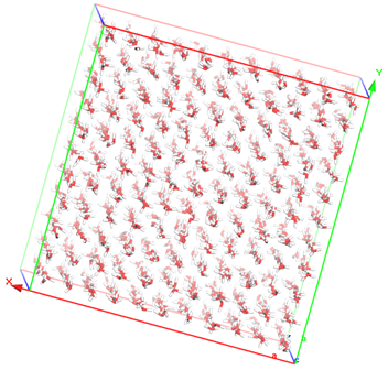
• Please view the PDB file using VMD or Movar simply by command:
  

  ./movar step2_solvbox.pdb

• Please view the energy profile by command:
  

  ./viewene step2_solvbox_min3.ene

  
  

 Step 3. Melting at 500k by command:

./modar step3_melt.inp nstep=500000

• Please read the scipt file "step3_melt.inp" for more details.
• The output files will be:
  

  Filename File Type Description step3_melting.log Text The log file step3_melting.trj Binary Trajectory in Movar binary format step3_melting.rst Binary The MD system state for resuming run step3_melting.rst.prev Binary The “backup” of last “rst” file, Modar make a backup for old restarting state when writing a new state for restarting run to deal some accidents like the storage run out off capacity. step3_melting.ene Binary The energies profile of MD simulation

• The MD timing information would be printed on screen like:
  

  <<Running 2500000 steps simulation with timestep 0.002 ps << Integrator: VVerlet << Ensemble: NVT << Thermostat type: Nose-Hoover << Temperature of reservoir: 500 K << Mass of virtual particle: 1000 <<  << Time escaped: 0.100591s for 10 steps <<  MD rate: 8.58924e+06 steps/day, 17.1785 ns/day <======== << Time Left: 6 hours and 59 minutes <<  << Time escaped: 0.866125s for 100 steps <<  MD rate: 9.97547e+06 steps/day, 19.9509 ns/day <======== << Time Left: 6 hours and 0 minutes <<  << Total size of the TRJ file will be about 229.00 Mb for 5.005 ns simulation <<  << Time escaped: 4.31613s for 500 steps <<  MD rate: 1.0009e+07 steps/day, 20.0179 ns/day <======== << Time Left: 5 hours and 59 minutes <<  << Time escaped: 60.3504s for 7500 steps <<  MD rate: 1.07373e+07 steps/day, 21.4746 ns/day <======== << Time Left: 5 hours and 34 minutes <<  << Time escaped: 799.044s for 97500 steps <<  MD rate: 1.05426e+07 steps/day, 21.0852 ns/day <======== << Time Left: 5 hours and 28 minutes

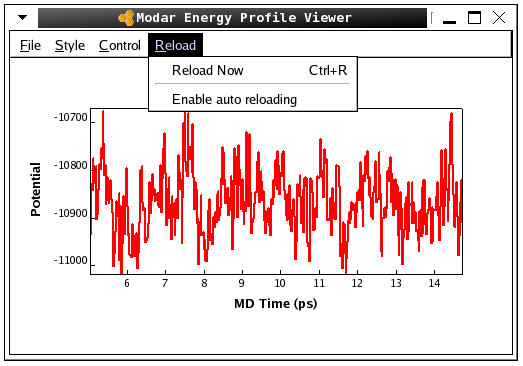
• Please view the trajectory "step3_melting.trj" by command:
  

  ./movar step2_solvbox.pdb step3_melting.trj

• Please view the energy profiles "step3_melting" by command:
  

  ./viewene step3_melting.ene

  Here is a snap of the fluctuation of totoal potential energy shown in Modar energies profile "viewene".

  
  

 Step 4. Equilibration at room temperature by command:

./modar step4_equil.inp nstep=1000000

• It will run a short annealing to 300K using Bereandsen temperature coupling, and do 2ns equilibation using Nose-Hoover thermostat to relax the system.
• Please read the explanation of the scipt file "step4_equil.inp" for more details.
  
• Or we may use "nstep=0" and it will build a MD core only stored in file "step4_equil.mds", which is a compact binary file contains all data and parameters for further MD simulation, and then copy the file to a HPC cluster and run the job using a MPI version modar by command:

mpirun <MPI arguments here> ./modar_mpi step4_equil.mds nstepmore=1000000

• The output files will be:
  

  Filename File Type Description step4_equil.log Text The log file step4_annealing.trj Binary Trajectory fie in Movar format on annealing stage step4_ annealing.rst Binary The MD system state for resuming run step4_annealing.ene Binary The energies profile on annealing stage step4_equil.trj Binary Trajectory file on equilibration stage step4_equil.ene Binary The energies profile on equilibration state solvbox.msf Text The final structure of the water box in Modar MSF format solvbox.pdb Text The final structure in PDB format

• "solvbox.msf" can be used as a raw unit for building a larger water box as shown in other examples.
  
• Please view the energy profiles by command:
  

  ./viewene step4_equil.ene

• Please view the trajectory by command:
  

  ./movar step2_solvbox.pdb step4_equil.trj

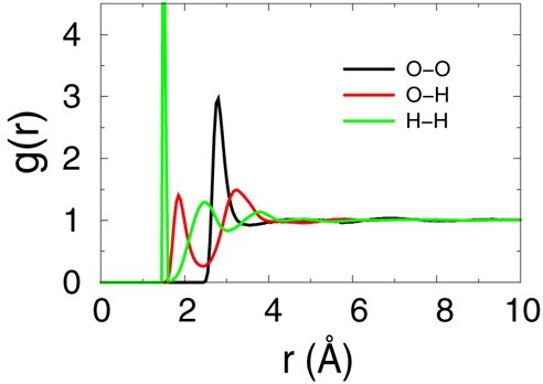
 Step 5. Calculate the radial distribution function by command:

./modar step5_calc_rdf.inp

• The raidal distribution function over the last 100ps samples will be evaluated to make sure that we got a well equilibrated water solvent box.
• Please read the explanation of the scipt file "step5_calc_rdf.inp" for more details.
  
• The output files will be "rdf_O_O.txt", "rdf_O_H.txt" and "rdf_H_H.txt". Please plot this 3files together using xmgr or gnuplut. The result should be simlar to bellow figure, which means the system is equilibrated enough according to reference [Structure and Dynamics of the TIP3P, SPC, and SPC/E Water Models at 298 K, Pekka Mark and Lennart Nilsson, J. Phys. Chem. A 2001, 105, 9954-9960].
  

 Summary

• In this practice, we generated a small water box with 1331 molecules by replicating from a single water molecule first; Then the pseudo-crystal was heated up to 500K and melted through 1ns NVT simulation; Then the system was annealed to 300K and being equilibrated for 2ns more with Nose-Hoover thermostat; Finally the last 100ps samples were used for radial distribution function (RDF) calculations, and the results indicated the water box is well relaxed.
  

 Computational detail

• The water box was built basing on CHARMM 27 Tip3p model in cubic shape with density of 1.0 g/cm.
• Berendsen weak temperature coupling method were used on both tempering and annealing processes.
• Nose-Hoover thermostat approach was used for keeping constant temperature in all NVT equilibrating simulations.
• All hydrogen relatived bonds were constrained through Shake algorithm in all simulation.
• The long range electrostatic interactions were evaluated precisely through PME algorithm, and the short range interactions were truncated at 10.0 angstrom with a switch function.
• All simulations were propograted using leapfrog integrator with a time step 2fs, and samples were collected for every 1ps second.